The SDSS will collect, process and distribute vast amounts of data. Indeed, the size of the data handling task is such that we could not reasonably have contemplated doing this survey even a few years ago with the compute power available then, even had all the other necessary technical developments (detectors, optics etc.) been in place. The task is far from trivial today, but it is doable; indeed, as we discuss in this chapter, the software is basically in place to run the survey.
The organization and processing of the SDSS data require techniques similar to those used in large high-energy particle physics experiments, and the entire data processing activity is managed by scientists in the Experimental Astrophysics and On-line Systems groups at Fermilab. Much of the science software is also written by these groups, but some self-contained tasks are being done at the member institutions, as described below, because of the presence there of small groups of people with talent in the appropriate area. These groups report their activities directly to the Fermilab group, change activities via negotiation with this group and maintain compliance with the data model, which contains the definitions of the data outputs and interface data for the Survey. The management activities will be described later in this chapter.
The data flow through the acquisition, analysis and archiving phases is organized according to the following principles:
| Spectroscopic | Photometric | Postage | Quartiles | Astrometric Stamps | |
|---|---|---|---|---|---|
| Bits/pixel | 16 | 16 | 16 | 3x 16 | 16 |
| Number of CCDs | 4 | 30 | 52 | 30 | 24 |
| Number of pixels per CCD | 2192x2068 | 2192x1354 | 40x29² | 2192x1354 | |
| per frame time | 18.1 Million | 89 Million | 1.7 Million | 71 Million | |
| Peak data rate per CCD | 153 kBy/sec | 153 kBy/sec | 1.9 kBy/sec | 340 By/sec | 153 kBy/sec |
| Average data rate | 48 kBy/sec | 4.6 MBy/sec | 99 kBy/sec | 10 kBy/sec | 3.7 MBy/sec |
| Raw data per night(10 hours) | 1.7 GBy | 170 GBy | 3.6 GBy | 360 MBy | |
| Total raw data | 360 GBy | 12 TBy | 254 GBy | 25 GBy |
Table 14.1 summarises the data acquisition rates and the total data storage requirements for the Survey. The meaning of some of the terms used in Table 14.1, and the assumptions used to calculate the data rates, are as follows. The data stream from each photometric CCD is cut into `frames', 2048 x 1362 pixels, for ease of handling in subsequent processing. The set of five frames in each of the SDSS filters for a region of the sky is called a `field'. We assume that we are reading from two amplifiers for each of the photometric CCDs, with 20 extended register pixels and 20 overscan pixels read through each amplifier, in addition to the 1024 data pixels, for a total of 1064 per amplifier. The extended register and overscan pixels contain no light signal and are used to establish the electronic zero points and baselines for the system.
The `postage stamps' are 29 x 29 pixel subimages of bright stars cut from the imaging data stream by the DA system, which are analyzed on line to monitor the image size and are also passed to subsequent data reduction. (Historical note: US postage stamps for first class mail cost 29 cents when this system was designed). Quartiles are taken of the data in each column for each CCD and are used for the construction of flat fields.
The quantity of spectroscopic data was calculated by assuming that flat field and wavelength calibration frames accompany each pointing and that the data exposure is split into three parts. This gives a total of about 160 MBy per spectroscopic frame, and we hope to complete one field per hour. We have assumed that two amplifiers are used for each spectroscopic CCD and that they are read by a split serial register as are the imaging CCDs and that, in addition, they have a 20 pixel vertical overscan, used to establish the electronic zero points and baselines.
We will not keep all of the data from the astrometric CCDs (which have a total data rate about 2/3 that of the photometric CCDs). There will be about 500 stars per square degree averaged over the survey region which will be bright enough for astrometry, and we will keep centroid and shape information, plus a 29 x 29 postage stamp for each star in each of the 22 astrometric CCDs separately. The `total data' entries include all of the overlaps, both between CCDs in a stripe and between stripes. We will keep postage stamp data from the focus CCDs just as we do from the astrometric CCDs for quality control.
The total amount of data to be gathered and archived by the SDSS is huge, and is dominated by the imaging data. The quantities listed in Table 14.1 do not take data compression into account. The catalogues will be stored in efficient format in the data base, and the images and postage stamps compressed. Gains of a factor between 2 and 3 are likely in storage efficiency. Further, as we discuss later in this chapter, we may implement the construction of highly compressed data cubes which can encapsulate a description of certain fundamental aspects of the survey data (e.g. the galaxy distribution for the entire survey) in much more compact form for subsequent analysis.
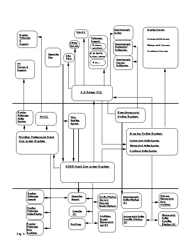
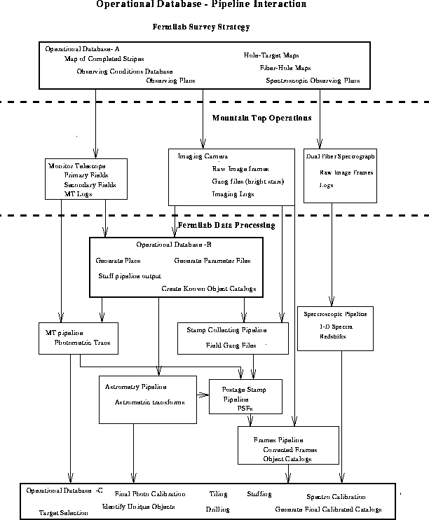
Figure 4.1 (in Chapter 4, Project Status) shows an overall schematic of the data flow in the SDSS from the sky to published astronomical papers. The software necessary to achieve this falls into two main categories, data acquisition and data processing.
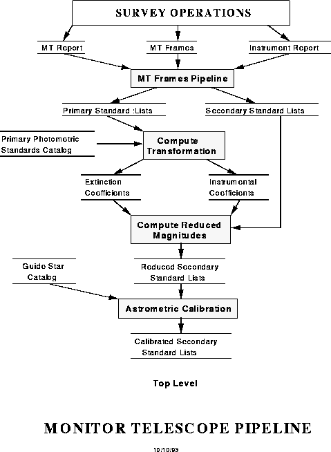
Figure 14.1 gives a simplified view of the Data Acquisition (DA) systems and how they interact with the instruments and the follow-on processing. We will have four major instruments to deal with at APO: the photometric array (30 CCDs), the astrometric/focus array (24 CCDs), the spectrographs (4 CCDs), and the monitor telescope (1 CCD). Each instrument has its own VME-based realtime control system with a backend UNIX workstation. The control systems have similar architecture and share much software, although each is tailored for its specific application. The photometric, astrometric, and spectroscopic systems share an SGI Crimson host computer; the monitor telescope system has its own SGI Personal Iris computer.
Top-Level Survey Operations
Data for a particular location in the sky will come from one column of CCDs (we define columns to be parallel to the scan direction, just as the columns of the chips are). The focal plane showing the photometric and astrometric chips is illustrated in Figure 8.2 (in Chapter 8 about the Camera). Each column of photometric CCDs is associated with two astrometric chips, a leading one and a trailing one which scan the same region of sky as the photometric column, the leading immediately before the first chip and the trailing immediately after the last chip of the photometric column. Between these astrometric devices are the astrometric bridge CCDs, of which there are also leading and trailing sets and which establish the astrometric link between columns. For the purposes of data acquisition and organization, it is convenient to divide the CCDs along slightly different lines; we will treat the CCD array as ten sets of CCDs. Each of six photometric sets contains the five CCDs from a column. The four astrometric sets consist of the four rows of astrometric chips. In each astrometric dewar the five "bridge" chips and the focus chip are one set and the six chips corresponding to the photometric chips the other. Thus there are six identical photometric sets of five chips, two identical astrometric sets of six chips, and two identical astrometric/focus sets of six chips. Each set has its own acquisition processor and communicates with it over a single optical fiber link.
The map of the sky will be assembled from data written in blocks of runs where each run corresponds to, say, 1 hour (although the length of a given run is arbitrary and will depend on observing conditions). A run covers a portion of a strip, and two interlaced strips are used to form a filled stripe. For planning purposes, we assume that there will be 45 stripes and 540 runs.
Figure 14.2 shows a diagram of the DA system that operates 3 columns of the photometric array (there will be two such systems for the photometric array). Data arrives from the telescope over a fiber optic link and is captured by a custom-built board (the VCI+). The data are then spooled onto disk in a `frame pool' that can store 45 minutes of data. This disk holding area is used to buffer data to cover tape drive failures. A scrolling display will show a portion of the data from one or more CCDs in realtime for diagnostic viewing. An MVME167C single board computer (based on a Motorola 68040 processor) handles one column of 5 CCDs. This computer will perform online processing as described below and will write the data to tape.
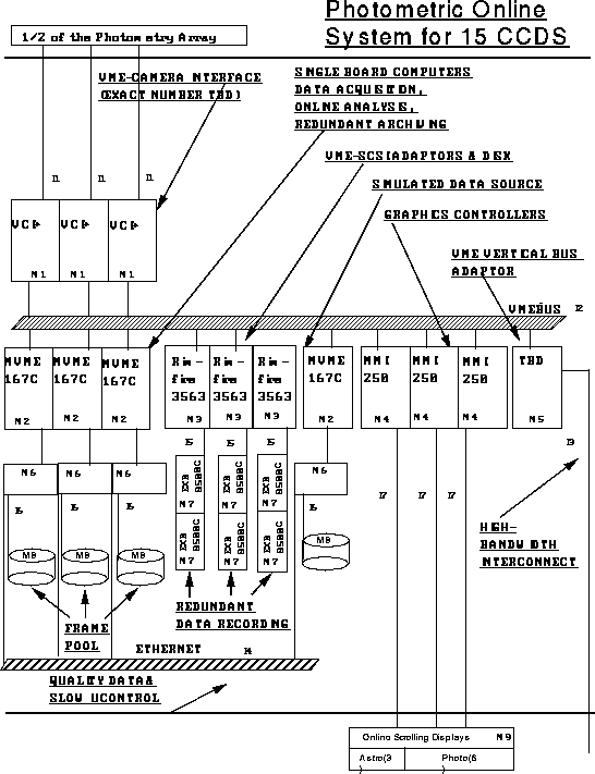
Online system for 15 photometric CCDs
We have chosen to use DLT 2000 tape drives to record the data. These drives combine high bandwidth with reasonable cost. A single drive can sustain a rate of 1 MBy/second, and a single tape can hold 10 GBy. The drives implement hardware LZW compression. We can record the data from a single photometric set of CCDs onto one tape, so we will run 6 DLT 2000s in parallel. Under dark sky conditions, the data will be compressible by at least a factor 2 using this algorithm, so the effective rate is ~ 2 Megabyte/second, more than adequate for the task. Because tape drives generically have reliability problems, we have chosen to record in parallel onto a second set of 6 drives; this will also provide us with a backup copy of the raw data. To ease the offline processing, the data from a single CCD are divided into frames of 1362 rows each (one half the separation between CCD centers) and recorded in a staggered fashion such that frames from the 5 filters for a given piece of the sky are written sequentially on tape. A set of tapes can record approximately 7 hours continuous imaging. The frame pool provides enough buffering to permit changing tapes without halting observing.
The processing of the data is split between the online system and the offline processing. The split is done for two reasons. First, if one simply recorded the data with no real-time processing, it would be impossible to perform even simple quality control procedures (What is the seeing? Are all the sensors actually working?). Second, there is information in the stream that is time-variable, (the forms of the PSFs due to seeing changes, focus and tracking imperfections, the sky brightness and color, etc) which may or may not be accurately determinable from a single frame, and for which in any case it is desirable to enforce continuity in the data stream. These quantities need to be extracted in a global way; part of this is done in the online processing and part offline, as will be described below.
The online system performs three steps of processing. First, the median, first, and third quartile points are computed for each column of pixels in a CCD frame (1362 rows). These quartile arrays are saved to disk. Second, a simple object finder identifies all bright stars with intensities that fall above some preset threshold, extracts 29-pixel square (12 arcsecond) postage stamps around each one, and computes shape parameters. These too are written to disk. In the subsequent processing, the quartiles are used to find the sky intensity and thus the flatfield vectors, and the stars are used for photometric, astrometric, and point spread function calculations. The data are also available to the observers and provide a convenient monitor of the sky intensity and seeing.
A full night of quartile vectors will occupy about 360 MBy of disk, and the postage stamps another 3+ GBy. One can now buy 9 GBy disks cheaply, so the volume of data can be handled without much trouble.
Data which are crucial to the calibration of the imaging data will be included in the data stream. These include the time; telescope pointing information; information about the health of the camera, including the chip temperatures and the readout noise derived from the extended-register pixels; and information from the Monitor Telescope regarding the seeing and transparency during the scan. Summary versions of these data will be recorded in a separate data base to facilitate the determination of long-term trends in the observing conditions and state of the instrument.
The DA system for the astrometric CCDs is nearly a copy of that for the photometric CCDs. However, only the postage stamps and parameters for the detected stars will be written to tape, not the raw pixel data from the astrometric chips. Over the survey region there are an average of about 500 stars per square degree bright enough for the astrometric chips to record to interesting accuracy, and these are the only ones in which we are interested for this purpose. For each of the stars we will record an accurate pixel position, shape parameters, a flux, and (just to cover ourselves) a 29 x 29 pixel (12 arcsecond) postage stamp of the star. By saving the postage stamps, we have the option to go back and apply flatfields and derive more accurate centroids using more complex PSF fitting at a later time, but we may well find that the improvement in centroiding is negligible. Each chip covers 9.4 x 10⁻⁴ square degrees per second, and so encounters about 0.5 of these stars per second; the whole array of 22 chips encounters about 11 per second. The DA will preferentially skip fainter stars if the rate for any CCD exceeds about 1 per second, given the CPU limitations of the DA computers, but that does not have any impact on the subsequent processing.
The data rates for the spectroscopic survey are much more modest, and consequently the DA system is much simpler than that for the imaging system. We will use the same basic architecture for instrument readout (a VME crate with an MVME167 control computer), but the raw pixel data will be sent straight to the Unix host computer for storage.
We have two double spectrographs, so the 640 spectra are recorded on four 2048 x 2048 CCDs. After an exposure we read out a total of 36.3 MBy (4 CCDs worth). The readout time in 2 amplifier mode is 59 seconds.
The spectroscopic exposures will probably be split into three parts to allow cosmic ray removal, and will be accompanied by calibration data, probably one flat field and one wavelength calibration (if the night sky lines plus occasional spectral lamp exposures do not suffice), which multiplies the total data and average rate by 5. There will probably also be some highly binned spectroscopic frames (taken with the telescope slightly offset to discover exactly where the fibers fall on the galaxies -- cf. Chapter 11.8), which add negligibly to the total amount of data. Thus each spectroscopic frame and associated data amount to about 180 MBy and simultaneous access to more than one frame is not necessary. The total amount of spectroscopic data recorded depends on the number of targets. If we assume that each spectroscopic field looks at 5 square degrees of sky (the full 3 degree round field is seven square degrees, but the inscribed hexagon is 6.2 square degrees and there must be some overlap to allow for adaptive tiling), there will be about 2000 spectroscopic fields, 250 eight-hour plus (for overhead) nights, and a total database of about 360 GBy. These data will compress by a factor of two to three, although compression seems hardly necessary.
Data that are crucial for the calibration of the spectra and their correlation to the photometric survey will be written along with the spectra. These include the time, telescope pointing information, and fiber placement measurements, as well as any engineering data which are relevant, such as chip temperatures and read noise.
The monitor telescope DA system is essentially a smaller version of the spectroscopic system, since there is only 1 CCD to be controlled. The monitor telescope will operate in a semi-automated fashion. The default observing program will be to observe a sequence of primary standard stars to monitor atmospheric extinction. While the 2.5 meter is operating, the monitor telescope will receive positions of secondary star fields to be observed as well. (These can be done any time, so long as they are available for reduction of the photometric data; and it would be advantageous to get ahead of the imaging survey.) We will be able to observe roughly 6 primary standard stars and 3 secondary fields per hour. For the primary standards, we will record only the central 1024x 1024 of each frame. The maximum amount of data that could be collected in one night is about 2 GBy. Again, these data will be stored directly to disk.
The primary standard star frames will be processed in real time in order to extract instrumental magnitudes. Calculation of a photometric solution roughly once an hour, and comparison of the measured and expected counts for each star, will allow us to determine the time period when the night is photometric; this information will be relayed to the 2.5 m observer in real time to facilitate planning of the night's operations.
The photometric, astrometric and spectroscopic DAs will share a backend UNIX host workstation (an SGI Crimson). This workstation will provide the operator interface to the DA system, provide compute power for any `quick look' processing of images that is not already being done in the VME computers, and provide displays of critical information on the system performance. Most of the key information that one might want can be extracted from the star lists and quartile arrays, and so the monitoring task is simply to format this information for the observer. The realtime analysis of the camera data is performed by a collection of routines called `Astroline'.
All of the control and analysis software is written using the TCL (Tool Command Language) based software framework that is described in Section 14.3.2.7. A common core DA system is provided for all the instruments, with the code split between the VME front end and the Unix back end computers. The common core DA can receive data from multiple CCDs, perform the online analysis tasks, spool data to disk and tape, run the scrolling displays, and pass information between the VME and Unix processes. Each major instrument has customized configuration files and TCL-based observing programs. The TCL language provides features such as multi-tasking, foreground/background process control, interprocess communications using TCP/IP, file I/O, X window GUI construction tools, and extensive interfaces to the Unix operating system. The observing program is broken into several processes that are run as independent tasks. For the imaging system, for example, the following processes are provided:
For the spectroscopic observations, we will use IRAF to perform any online analysis (e.g. quick flatfielding, extraction, wavelength solutions) as required.
The bulk of the data processing will be done offline at Fermilab. Tapes from a night's observations will be shipped via Federal Express (which picks up at the Observatory). We feel that this approach is preferable to the alternative of doing the processing on the mountain, the reasons including the difficulty of maintaining the fairly large computing system required for the reductions and the necessity in any case of getting the data to the central archive. The effective baud rate of a box of DLT tapes carried by Federal Express is much higher and the transfer much more reliable than that afforded by current network protocols.
There are several constraints on the data processing that must be met. The imaging observations must be reduced in a timely fashion in order to identify spectroscopic targets. Ideally we would like to turn around the image processing on the time scale of a few days, but there are enough steps involved that this may not be practical; furthermore, a given spectroscopic plate will require of order 6 separate stripes to be combined in order to generate target lists if we are to take advantage of the benefits of adaptive tiling (see Chapter 12). Practically, we will aim to have all imaging data from a given dark run reduced in time to have spectroscopic targets available for the next dark run -- this gives us a required turnaround time of about a week. Given the large amount of data that must be processed, and the desire for uniformity, the algorithms must be sufficiently robust that minimal human intervention is needed. Finally, rapid turnaround is needed to verify the quality of the data and allow re-observation of a given field if necessary. Thus we will have accomplished our most fundamental goal the code implemented at the beginning of the survey correctly finds and classifies all spectroscopic targets. If, furthermore, we find all the objects present in the data to the desired significance level and extract large enough subimages on the first pass, we need never return to the full pixel data set for reprocessing, and can do improved processing on the much smaller subimage data set (cf., the discussion below in Section 14.3.5.10). However, if we find it necessary, we will be able to reprocess the imaging data (though we will go to great lengths to avoid having to do so), as long as it does not affect the spectroscopic selection.
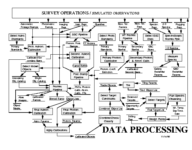
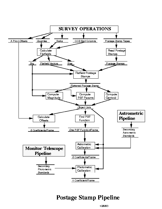
Figure 14.3 gives an overview of the complete data processing system. Each tape of raw data from the mountain is fed into a "pipeline" that performs routine processing and produces some output, usually of much reduced size. The astrometric, monitor telescope and photometric pipelines are very interdependent. The astrometric and monitor telescope pipelines are fairly straightforward to design and implement, but the pipelines that process data from the photometric CCDs present the greatest problems because one needs calibration data available in order to process the data, but final calibrations, especially quantities like the PSF parameters and the flat field as a function of time, are not local quantities, and are thus not available until well into the pipeline processing. We have addressed this problem by breaking the processing into two stages: the `postage stamp' pipeline and the `frames' pipeline. The postage stamp pipeline takes the postage stamps of bright stars and quartiles that were extracted from the online system and the upstream Serial Stamp Collecting Pipeline and computes the flat-field vectors, point-spread functions, and gets Monitor Telescope calibration lists and an astrometric solution, sufficient for the frames pipeline to function in such a fashion that individual frames can be processed independently. The output contains sufficient information about each object that it is possible to derive and apply slightly revised calibrations after the fact. The six columns of CCDs are independent of one another for the purposes of data processing, so our pipelines are designed to process one column of CCDs at a time.
The overall SDSS management and organization structure are described in Chapter 16, but those relevant to the software organization are briefly summarized here. Since the software is designed for automatic reduction, cataloguing and archiving of the vast SDSS data stream, it is largely via the software pipelines, in particular the code which selects the spectroscopic targets, that the scientists at the SDSS institutions carry out the scientific design of the survey.
The SDSS is driven by the requirement to carry out its observations in a uniform, accurate, well-controlled, well-documented and well-understood manner. As the software has evolved, it has proven most effective to place responsibility for each of the major software pipelines in the hands of a small group whose members, as far as possible, are located at the same institution. Almost as important as the development of the software is its testing, and this is organized so that the pipeline development is done by one group and tested by another. The institutional responsibilities are:
By making use of extensive simulations, we have managed to demonstrate that all of these pipelines are able to interoperate. Specifically, we have run 10°x10° of simulated data through the entire system, up to and including target selection. This is a non-trivial achievement, and we periodically repeat the exercise to confirm that no inconsistencies have appeared.
With so many people working on the software at so many locations, it was clear that some sort of software management tool would be essential. We have chosen to use the well known free product CVS, which has proved to serve our needs well. The code repository is resident at Fermilab. Specifically, CVS allows:
The prototyping of the pipelines is, basically, a proof-of-concept exercise, and was carried out for the photometric, astrometric and spectroscopic pipelines only. These pipelines were written in outline form to analyze a small set of data which are not fully self-consistent and are far from reflecting the true system complexity (e.g. this software dealt with simulated data from only five photometric CCDs and one astrometric CCD; further, there was no requirement that the outputs be scientifically valid). The data base was used at this stage only in the development of the spectroscopic pipeline.
Level 0 is a test data processing system that is designed to ensure that the data procession framework is working correctly. The pipelines completed to Level 0 on the above date were the photometric, astrometric, spectroscopic and monitor telescope pipelines. They contained most of the necessary functionality and operated on a set of self-consistent test data. The imaging data pipelines were fully integrated, and the outputs were scientifically meaningful.
Data flow through the imaging and spectroscopic pipelines.
This system is as complete as possible without having actual data from the telescope. It is designed to have full functionality, i.e. to be able to run the survey, and operates on a set of simulations which have been designed to be as realistic as possible. The imaging pipelines (monitor telescope, astrometric and photometric) have been fully integrated, run efficiently and exhaustively tested, while the spectroscopic pipeline is ready to be integrated in early 1997. The imaging pipelines produce meaningful scientific output which has been successfully used to run the target selection pipelines and science and operational data bases.
This is the software which will carry out the data reduction for the entire survey. During the test year (Section 5.3), the algorithms will be optimized for real data. Level 2 will be "frozen" at the beginning of survey operations proper.
As will be seen in the discussion of the individual pipelines below, the functionality is usually provided by several sub-pipelines. The pipelines are coded in ANSI-C and TCL, and are built on a basic framework developed at Fermilab called DERVISH/SHIVA (the latter was the name until December 1996, hence the nomenclature in some of the figures in this chapter - it's a long story). The Astrometric (ASTROM), Monitor Telescope (MTpipe) and Photometric (PHOTO) pipelines are integrated under DERVISH/SHIVA and run together to reduce a night's worth of photometric data - see Figure 14.3. The task of maintaining this operating environment and of integrating the pipelines and maintaining the integration is a major one. A very large amount of code is involved in ensuring that the pipelines talk to each other and to the data base, in monitoring the processing tasks and ensuring that the outputs from the processing are available when needed. Furthermore, the software must be embedded in a framework which provides image displays, command interpreters and so forth.
The online system detects bright stars above some preset threshold and saves both a postage stamp and the image centroid and shape parameters. No flatfielding is done. The present astrometric pipeline makes use only of the image parameters; processing of the postage stamps will be added later if deemed necessary. The centroiding algorithm makes use of the fact that the image of a point source is roughly Gaussian. The data are smoothed and interpolated using the standard seeing model approximation of a two component concentric Gaussian, the outer component having 1/10 the amplitude and about twice the width of the inner. Information useful for astrometry is contained entirely within the inner component. The centroid is then found by fitting a corrected polynomial expansion of the central Gaussian to the marginal x and y distributions of the data. The accuracy of this computation is < 3 mas due to systematic effects and ~ 20 mas due to photon noise at 20th magnitude. This is much better than the errors expected from classical seeing theory (Section 10.4.2) of about 30-40 mas. The identical centroiding algorithm is used in the Photometric pipeline (see below) to ensure that the astrometric information is properly transferred to the photometric data.
Architecture of the Astrometric Pipeline
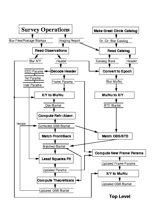
Figure 14.4 shows a diagram of the astrometric pipeline. The major steps in the process are as follows:
The retained output of the astrometric pipeline therefore is a calibrated position for every observed star, a set of 6 coefficients for every photometric frame in the run. There will be in addition a detailed record of the reduction process and a large set of parameters from the least squares fit that will be archived, although they will not be used further.
The purpose of the Monitor Telescope Pipeline (MTpipe, or MT for short) is: (1) to measure the extinction at the site as a function of time and (2) to calibrate the secondary standard stars across the sky (see Chapter 9). These secondary standards are thereby tied to a small network of primary standard stars (Fukugita et al. 1996). This is done using semi-autonomous observations of standard stars and secondary standard calibration fields (see Chapters 5 and 9). The data flow through MT is shown in Figure 14.5. MT automatically reduces these observations and makes the measurements which the photometric pipeline needs to calibrate the imaging data.
Data flow through the Monitor Telescope Pipeline.
MT consists of three sub-pipelines: MTframes, Excal and Kali, which are invoked in this order. MTframes, analogous to the Frames routine in the Photometric pipeline, does the bulk of the reduction of the raw MT data on a frame-by-frame basis. It bias-subtracts and flat-fields the data, searches for objects, measures them and outputs the results.
Excal is a TCL procedure which performs the photometric solution by a least-squares fit to the output of MTframes. To do this it must identify the standards automatically from the frames. This routine works on the primary standards, and outputs extinction measures for the Postage Stamp Pipeline (part of the photometric pipeline; cf. Section 14.7) to work with.
Kali is a TCL procedure which applies both a rough astrometric solution and the photometric solution to the secondary standards to run as input to the Postage Stamp Pipeline.
The photometric pipeline (PHOTO) is required to carry out the following tasks:
Correct the Data: Flat field, interpolate over bad columns, and remove cosmic rays
Find Objects: Sky level measurement, noise measurement, sky subtraction, object finding
Combine Objects: put together the data from the five bands for each object.
Measure Objects: position, counts, sizes, shapes
Classify Objects: provide parameters for object classification, i.e. goodness-of-fit parameters from fits to simple models (point source etc.)
Deblend Objects: do simple model fits to overlapping images.
Output Results: Write out an object catalogue plus images and corrected data.
The pipeline operates on a frame by frame basis. The photometric data stream from each CCD in the photometric array is cut into frames of 2048 x 1362 pixels. Frames are then re-assembled by adding to the top of each frame the 128 rows from the next frame, so that the frames before processing are 2048 x 1490 pixels with 128 pixels overlap with the next frame. The five frames for each field are then combined. (Note that the individual bands are observed sequentially.) This is the same number of pixels in the side-to-side overlap when the two strips of a stripe are observed. Each set of five frames is then processed. However, as we mentioned above, the processing needs information for the entire run: quantities such as the point spread function, the sky brightness, and the flat field and bias vectors are not local quantities, but are determined as a function of time, smoothed where appropriate, and interpolated to each frame. This requires at least two passes through the data, and thus PHOTO consists of three pipelines. In order of execution these are:
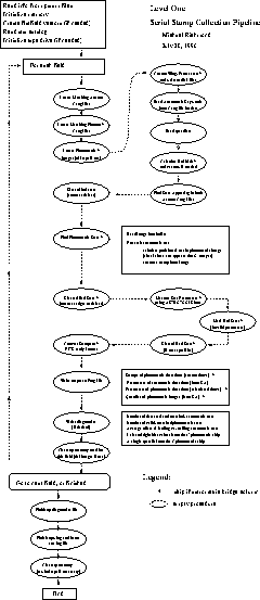
Serial Stamp Collecting Pipeline (SSC): cuts out postage stamps (currently 65 x 65 pixels) from the photometric data stream for input to the PSP, and orders these files in an appropriate format.
Postage Stamp Pipeline (PSP): analyzes these postage stamps, and characterizes the point spread function from these images. It calculates the bias, sky and flat field vectors for each row. It also takes input from the astrometric and monitor telescope pipelines to calculate preliminary astrometric and photometric solutions.
Frames Pipeline: Performs the analysis on the frames one at a time, using calibration information from the PSP.
PHOTO uses this architecture because the frames pipeline is very compute intensive. The architecture allows the Frames pipeline to run for one set of frames at a time regardless of the ordering of the frames - the calibration and instrumental information for the entire scan is carried by the Postage Stamp Pipeline. The compute engine for the production system is a multi-processor DEC Alpha (see below) which can run multiple copies of Frames, and pass a new set of frames to each processor asynchronously as the processing of the previous set finishes. Although the PSP originally used only the postage stamps cut by the DA system, further development showed that if postage stamps were cut from the imaging data for the stars detected by the astrometric CCDs, both the astrometric and photometric solutions are greatly improved, which prompted us to write the SSC. This, however, necessitates two passes through the data. As will be discussed below, we have fast enough machines and code to allow this.
Flow diagram for the Serial Stamp Collection Pipeline
Figure 14.6 shows the architecture and data flow for the Serial Stamp Collection pipeline (hereafter SSC). The first job of the SSC is to cut postage stamps for three categories of star from the photometric data and to pass them to the PSP and Frames pipelines. These are: (1) stars detected by each pair of leading/trailing astrometric chips. The postage stamps are 65 x 65 pixels. (2) one 200 x 200 pixel postage stamp from each frame around a star brighter than 14m (the central part of the image will be saturated). These stars are bright enough that they will show first order ghosts due to internal reflections in the camera optics. (3) an entire frame every hour or so containing a star brighter than 7m ; these stars are bright enough to show ghosts due to secondary reflections in the camera.
Stars in category 1 serve two purposes; they allow the point spread function to be measured and they allow the astrometric solution to be transferred to the photometric data. To this end, the parameters of the unsaturated stars (centroids, widths) are measured using exactly the same code as does the online astrometric DA system. The outputs of the SSC are written to an output file for use by downstream pipelines.
The online DA system reads out each CCD in the imaging camera and groups together data from all of the images read out at one time into an output file. Since it takes about 10 minutes for a star to cross the astrometric and photometric arrays, the images in this file do not correspond to the same area of sky. The second purpose of the SSC is to re-arrange the DA data stream so that all of the data for a given piece of sky are collected into a single output file. The frames in the five different bands for the same part of the sky are called a field.
Flow diagram for the Postage Stamp Pipeline
The data flow through the PSP is shown in Figure 14.7. The PSP calculates the bias vector, flat-field vector and point spread function (PSF) and interpolates them to the center of each frame. It uses bias and data quartiles produced by the DA system and an input file describing each CCD, which contains information on bad columns etc., which are used to interpolate the data in the postage stamps. The postage stamps from the SSC are filtered for unsuitable objects (saturated stars, galaxies) and the point spread functions calculated by fitting a classified PSF model to the image, as described above in Section 14.3.3. The composite PSF for each frame is then calculated from the weighted mean of the PSF star data in that frame. If there are not enough PSF stars on a given frame (a likely occurrence in the u' band at high galactic latitudes) the mean PSF is found from the stars in several frames and interpolated to the center of each frame. The frame correction and calibration vectors are calculated from the input quartiles and overclock data. The outputs for each band are: a bias vector for the entire imaging run; a flat-field vector for each frame; bias drift values from both amplifiers in each frame; the sky value for each frame; and the sky gradient for each frame.
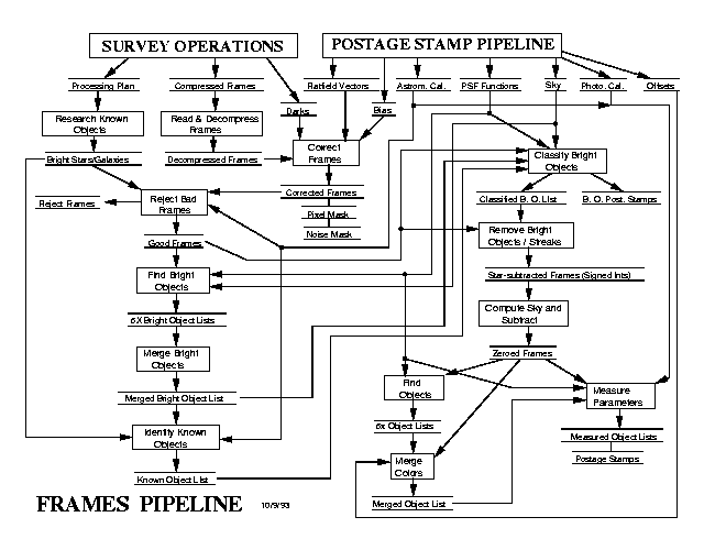
Flow diagram for the Frames Pipeline
The Frames pipeline operates on one set of frames (a field) at a time. The following is a much simplified outline of its operation (see Figure 14.8):
The inputs required by Frames are: the CCD hardware specifications (locations of bad columns etc.); raw frames in each color with overlaps attached; bias vector for each CCD; flat field for each CCD; model PSF in each color; calibration data (the approximate flux calibration, and coordinate transformation for aligning the pixels in each frame to the fiducial frame, r' , because the astrometric CCDs observe in this band).
First, the frames are flatfielded using the flat field found from the data quartiles in the PSP. They are then corrected for defects. Three types of defect are corrected by interpolation: bad columns, bleed trails and cosmic rays. The survey CCDs are required to have any defects no more than one column wide, for which almost-perfect interpolation is possible because the pixel size samples the PSF at the Nyquist limit. The interpolation algorithm can also treat defects more than one column wide, such as bleed trails; however, these can be only partially recovered.
Interpolation over bad columns. The upper panel shows simulated images of a bright star with a bleed trail and a bad column just to the right of the trail. Lower panel: interpolated and corrected image. The faint object just above the center of the bright star has been recovered.
The correction of bad columns is done using linear prediction (see Press and Rybicki 1993 for a discussion) to interpolate the data across pixels where it is missing. This is done by calculating the interpolation coefficients for a seeing-convolved point source, i.e. the PSF, sampled by the pixel response function of the CCD. These can be calculated directly in the case of noiseless data, and the value at the location of the missing data interpolated using data on either side of the bad column(s). The algorithm used by PHOTO uses +- 2 columns on either side of the bad column, and, for bright stars containing a one-column defect, recovers the flux to about 1%. This method cannot be used for wide defects, such as bright star bleed trails; for these, the mean of the 2 values on either side is used. Figure 14.9 shows the correction of a frame with bleed trails and one bad column.
Cosmic rays are corrected in an analogous way. We do not have more than one frame of a given region of the sky, so cosmic rays cannot be found by comparison of two images in the same field. Rather, they are found because their signal is outside the band limit, i.e. the difference in counts between two adjacent pixels is larger than allowed by the PSF. Cosmic rays are found by comparing the intensity of each pixel with those of its eight neighbors, and removed by interpolation as described above. Information as to which pixels in an image are replaced with interpolated values is recorded in a mask image (which is highly compressible and therefore makes minimal impact on the data storage requirements).
Object finding is done in two stages: find (and remove if stellar) bright objects; and find faint objects. The reason for this two-stage process is that bright objects have large scattering wings, which on average cover something like one third of the sky at the 1-electron level in the Survey images. Since all object finding is done by threshholding, this could result in very different efficiencies for finding faint objects, especially close to the limit, as a function of position on the sky.
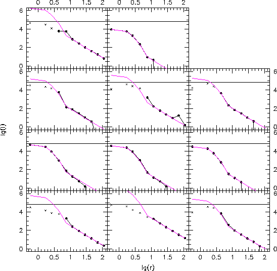
Radial profiles of bright stars. The ( r' band) data are from a simulated photometric frame. The filled circles are those used to derive the composite profile, and the crosses mark points that may have been contaminated by saturation. The horizontal line is the saturation level. The magenta line shows the derived composite profile scaled to the data.
Since objects are found by the standard threshholding technique, the data are first smoothed with the PSF, to optimally detect stars. The mean sky level and noise are found by median-filtering the frame, and bright stars found by threshholding at a high level (currently 60 sigma , about 16m ). The bright stars so found are then removed by modeling, fitting and subtracting.
The aim is to remove the power-law scattering wings around bright stars. To do so requires constructing a model PSF which consists of (currently) two Gaussians plus power-law wings. Constructing this model PSF is complicated, however, by the large dynamic range of the data: stars which are bright enough to have power-law wings whose measurement is insensitive to the sky level are saturated in the core of the profile, while unsaturated stars, for which the core PSF can be measured, are not bright enough to have measurable power-law wings. Accordingly, a composite profile is measured by fitting together observations of saturated and unsaturated stars. Figure 14.10 shows profiles derived this way. These fits allow determination of the fluxes of even saturated stars. Tests with simulated data show that we can determine magnitudes accurate to 5% for saturated stars to about 12m .
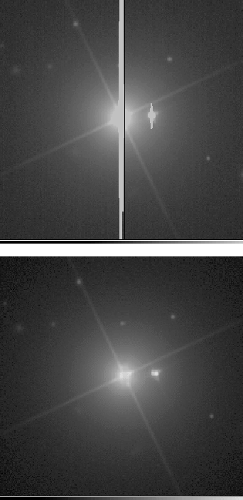
Figure 4.14 in Chapter 4 (Current Status) shows the result of fitting and removing a bright star. This subtraction is done to roughly 0.5 DN, with suitable dithering to obtain proper noise statistics in the other parts of stars. Note that some of the faint objects in the star's wings are found as `bright' objects because they are sitting on top of the bright wing and contain enough counts to be detected at the bright object threshold.
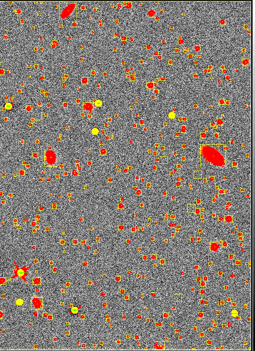
Object finding. A sample simulated r' frame is shown. Pixels deemed to belong to an object are colored red. Yellow pixels are the masked central regions of bright star images. Other masked pixels (measured to be saturated) are colored green. Squares are drawn around each detected object. There are also several blank fields to be observed by sky fibers during spectroscopic observations.
The corrected frames output by PHOTO will have bright stars removed. The parameters describing each star will be stored in the data base, so that the unsubtracted frame can be reconstructed if desired.
The object finder is now run again to detect faint objects. These are found as connected regions of pixels which lie above a given threshold. Since the data have been smoothed with the PSF, point sources can be single pixels at the limit.
The faint object finder is designed to work to the detection limit of the data. Its performance has been extensively tested by the JPG using simulations, and the algorithm works as theoretically expected; at magnitude 23.2 in the sensitive bands ( g', r', i' ) the point source detection rate is about 50% and the contamination rate less than 5%. The detection and contamination rates depend of course on the threshold level. The optimal threshold can be fine tuned using simulations, and will be fixed during the test year when data from the imaging camera have been extensively run through PHOTO.
Figure 14.11 shows the results of object finding in a simulated r' frame. PHOTO also identifies several regions per frame with no detectable stars or galaxies. These `sky objects' are to be used to locate the fibers which measure the sky spectrum during spectroscopy.
At this stage PHOTO outputs the corrected frames and masks as described above, and a 4 x 4 binned frame (which is both useful for searching for low surface brightness objects and carries sufficient information about the noise characteristics of the data).
In preparation for measuring the object parameters, PHOTO now merges the detections of the object in all five bands. To do this requires the coordinate transformations between the CCDs in each band from the astrometric solution.
PHOTO first measures the centroid in each color by fitting the PSF. The image is then shifted by sinc-interpolation so that the center lies at the center of a pixel, and the radial brightness profile measured. To keep execution time to a minimum the shifting is done only for the inner ~ 5" in radius; the outer pixels keep their original values.
We measure the azimuthally averaged radial profile by measuring the mean and median of the data in a set of concentric logarithmically spaced annuli centered on the center pixel. The median rejects, say, bright stars projected onto an extended galaxy. However, this calculation fails for the case of highly elongated objects (e.g. edge-on galaxies) because the median value within an annulus will just be the sky. We could use the mean instead of the median, but this would make us very sensitive to poor deblending of overlapping images. Accordingly, we go one step further: each annulus is divided azimuthally into 12 sectors. Medians are calculated within each sector, and the radial profile is then the mean of the twelve sectors. Tests have shown that the resulting profile is robust to inclination, as well as various forms of contamination.
The ellipticity and position angle are measured within the 1 sigma circular boundary by calculating the intensity-weighted second moments of x/r and y/r. Several flux densities are measured: the best-fit point source flux (by fitting to the PSF); the 50% and 90% Petrosian fluxes and radii (see the discussion in Section 3.1.2.4); the flux within a 3" aperture (the spectroscopic fiber diameter) under a fiducial seeing, and an isophotal shape, with the exact isophote level to be decided on during the test year. These aperture fluxes are all calculated by sinc-interpolation to properly account for the pixellation. The various fluxes are calculated in all bands, including those in which an object is not detected, to give a proper and consistent statistical description of the data in all five bands.
This last raises issues with representation of the data, because we will determine quantities like " -2+-4 units" which cannot be represented as magnitudes. Neither do we want to record linear units (Jy) because of the very wide range in brightness of real objects. We will likely use a pseudo-magnitude, i.e. "m" = A + B x sinh-1(F) , a quantity which handles negative numbers, is linear for small F and tends to a logarithm for large F.
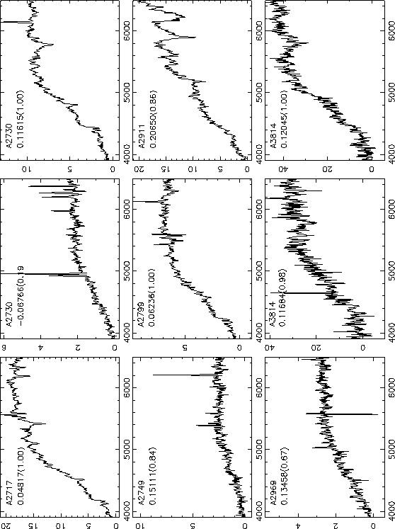
We now fit the median counts in the sectors to three simple radial profiles; a point source, a declining exponential and a de Vaucouleurs (1948) profile. This is done by a precalculated library of these functions with a range of scale lengths and inclinations, smoothed by the appropriate PSF. The best fit model parameters (peak flux, scale length, inclination, position angle) and the likelihoods are stored for each of the three types. The likelihoods can then be used to do a simple classification: star, spiral galaxy or elliptical galaxy. Any fancier classification or fitting, such as a bulge-disk decomposition (cf. Chapter 3.4) will likely await the development of off-line pipelines to further manipulate the data, as described below in Section 14.3.5.10. In any case, this is the method we use to do the star/galaxy separation. Extensive tests on simulated data show that this classifier works well essentially to the data limit, as shown in Figure 14.12. The object classifications are shown as a function of their `real', i.e. input, type. In Figure 14.12 object likelihoods are plotted; an object lying at the `star' location is a point source, one halfway between `exponential' and `de Vaucouleurs' is extended but equally likely to be a spiral or elliptical galaxy, and so on. The vertical axis of the classification "prisms" is goodness of fit, ranging from 1 at the bottom to 0 at the top.
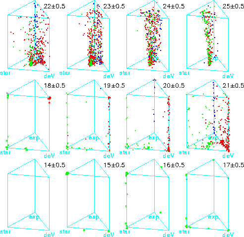
Performance of the object classifier. This is shown as a function of magnitude in g' , using simulated data. Green = input star; blue = input exponential disk; red = input de Vaucouleurs profile. The points corresponding to each object are located according to the model which best fits their radial profile. The vertical axis is the a measure of goodness of fit, with good fits at the bottom, and poor fits at the top.
Once a model galaxy profile is calculated, it is a simple matter to calculate a total flux. We believe that this is not likely to be a reliable flux because of template mismatch etc., but it is likely to provide good global colors. We will work these out by using the best-fit scale length in one band (probably r' ) to fit the peak amplitude in all five bands, and calculate the colors from these. These colors are of particular importance for determining photometric redshifts (Section 3.1.4.2). We have learned the obvious from this work; the PSFs must be very accurately represented in order to make good fits. It remains to be seen what will happen when we get real data.
Further structure parameters under development are some kind of texture parameter, calculated from the residuals left from inverting an image and subtracting it, and the representation of a radial profile as a series of orthogonal functions (PSF, de Vaucouleurs, exponential) which may allow the fraction of light in a point source nuclear component to be defined as a function of color and be a powerful diagnostic of AGNs and fuzzy quasars.
Finally, overlapping images will be deblended using the above models. During object finding, overlapping images are tagged (there are interesting problems associated with the different level of overlap in the different bands). They are then deblended using object models as above to estimate the total flux in each object. The parameters for both parent and child objects are recorded in the data base, appropriately flagged.
The result of these calculations is a large output file containing a catalogue of objects with a large number of measured parameters and uncertainties, plus pointers to the atlas image for each object. These outputs will be stored in the operational and science data bases. The nominal performance goal is to allow the robust and carefully controlled selection of spectroscopic targets, but these data will obviously enable a vast amount of science. There has been a very large amount of fundamental algorithm development for this work; the code will be made available to the scientific community and a detailed description of the algorithms will be published. Descriptions of many of these algorithms have been written up as internal documents (Lupton, 1993-6).
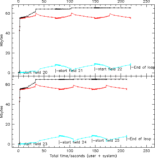
PHOTO performance. The graph shows the memory usage in MBy versus CPU time for a run of six fields, five frames each, on an SGI Origin 200. Black: total memory allocation by PHOTO. Red: memory usage. Blue: residual. The executable occupies another 15 MBy approximately. The two panels show the outputs of the two processors.
Atlas images are cut and stored for each object. Atlas images are subimages of size sufficient to contain the pixels belonging to the object, and the dimensions are set at the 3 sigma threshold, plus a border whose width is approximately that of the PSF. Unsaturated stars are thus well contained in a 29 x 29 pixel postage stamp. The dimensions of the atlas image for an extended object is set by those for the band in which the object is largest. Note that we cut an atlas image in all bands, even if we do not detect the object in all bands. Atlas images are also cut at the positions of sources from selected catalogues at other wavelengths (e.g. FIRST and ROSAT; cf., Section 2.1), whose positions are fed in from the data base on a frame by frame basis, with coordinates translated to pixels using the results of the astrometric pipeline. We will plan to cut these images without checking whether an image already exists because an optical object has been detected at that location; it is simpler this way and we can afford the overhead in storage required. Further, because objects look so very different at different wavelengths, it is useful to have an image cut to a size defined by the size of the object, e.g. it is likely that a larger image will be cut for a double-lobed `FIRST' source than would be cut for its associated optical galaxy. Further analysis which requires images of a larger area (e.g. searches for low surface brightness emission at large radii) can be made using the 4 x 4 binned frames.
As well as scientific and numerical accuracy, a prime requirement of the pipeline software is that it be robust and efficient in its use of memory and CPU. PHOTO handles the largest amounts of data in the SDSS by far, and it must be able to keep up. Development of fast, efficient code has been a prime concern; the calculations are done in integer arithmetic, memory allocation and use is very carefully controlled, and PHOTO operates on multi-processor machines in essentially parallel mode; fields are passed to processors as they finish the previous field independent of their ordering in the sky. The imaging survey takes data at 5 MBy/second; Figure 14.13 shows the memory and CPU usage by PHOTO running on a 2-processor SGI Origin 200 machine. Six fields (all columns of the camera) take 200 seconds to reduce on this machine and took 40 seconds to acquire; thus execution on the production machine, a DEC Alpha with 10 processors each roughly as fast as the individual SGI processors, can reduce the data essentially at the rate it was taken. Given the fact that the longest night's observing occupies only a third of 24 hours, and that photometric data can be taken only for a few nights a month, is is clear that the software and hardware are in place not only to keep up with the photometric data flow but to reduce it many times, if need be.
The entire focus of the photometric pipeline to date has been on readiness for the analysis of the Northern imaging survey; to analyze the photometric data rapidly, reliably and accurately enough that the reduction can keep up with the data rate, spectroscopic targets can be selected, and the performance of the imaging camera and of the conduct of the Survey can be monitored. Therefore, although the spectroscopic targets are brighter than 20m , we have ensured that objects are detected to the limits of the imaging data; these data are scientifically interesting, but more immediately they are a powerful diagnostic of imaging performance. Further, were we not to find objects to the limits of the data, the entire raw data would need to be reprocessed at some future time with different software. However, we have paid minimal attention to the processing of the data for the largest (D > 1' ) galaxies, which have internal structure of considerable scientific interest, given the difficulties of dealing with frame edges (cf., the discussion in Section 3.4.2). For these objects PHOTO will find the centroid, cut atlas images, and tag them as a `large' galaxy for automatic spectroscopic observation (Section 3.1.2.4). For the same reasons, the Southern photometric data will initially be processed like the Northern data - all imaging data will be run through PHOTO and separate object catalogues produced for each separate observing session.
Once PHOTO is developed to Level 2 and the Survey is well underway, further software development will take place. The following tasks, which do not affect survey operations, allow us to carry out further scientific goals of the survey.
The Southern imaging survey will repeatedly scan strips of the sky (Section 5.5), and to exploit the increased depth afforded by these data they must be co-added. This is not straightforward because data from different nights will not exactly map onto each other and each night's data must be fit to the cumulative coadded map before being added in. This fitting will also, however, allow us to add in data taken under non-photometric conditions, since it can be accurately calibrated by fitting to photometrically accurate data. We can therefore use more of the time for photometry in the South than we can in the North.
Just as we wish to co-add individual exposures on the Southern stripe, so too do we wish to carry out subtraction between them. Although many variability and proper motion studies can be done can be done at the catalog level, if we wish to search, for example, for supernovae close in to the cores of galaxies, we will need to be able to subtract "before" and "after" images of the galaxy from one another. This probably can all be done with Atlas Images, rather than having to go back to the corrected frames.
It will be of interest for many reasons to build a compressed version of the object catalogue as the survey progresses, to enable science analysis of several kinds. If each object found by PHOTO is described by a series of indices (position to a few arcseconds accuracy, magnitude to 0.1m - 0.5m , colors to 0.1m and, for galaxies, color redshift) we can build up two cubes describing the density of stars and galaxies in summary form. The stars cube describes color and magnitude distributions as a function of position in the sky and can be used in quasar selection as well as star count, cluster finding and correlation studies. The galaxy cube can be searched for clusters (it will be interesting to see how many galaxy density enhancements coincide with X-ray sources and with Bright Red Galaxies) and may be adequate for many statistical studies of large scale structure. The PHOTO group has developed code to construct and analyze these cubes (Kepner et al. 1997); the code will be incorporated into the data base at some suitable time.
The description of target selection above discusses how the object catalogues produced by PHOTO will be merged. We plan also to merge the reduced frames into a continuous five band image of the sky and to provide tools to access any part of it.
A second map which can be made as part of the development of the Merged Pixel Map is the sky map with all detected objects subtracted. This can then be searched for extended, low surface brightness objects.
The atlas images of the brightest, largest galaxies are likely to be of widespread interest. As described above, we will not engage in any extended analysis of these images in the routine data processing, but plan to investigate automated morphological analysis of the images, to produce analytical classifications, radial color profiles, color maps etc of a very large number of galaxies, to relate their morphological properties to the underlying dynamics and stellar populations. If this effort is successful, we can investigate the robustness of the classifications by degrading the images to simulate the effects of distance and redshift, as described in Chapter 3.4. This effort may allow a real comparison between the properties of nearby and distant galaxies.
Processing the imaging data for the Southern Survey will be substantially more complex than processing that for the Northern Survey. The DA system remains the same, though. The imaging for the Southern Survey has two main goals; to find variability from scan to scan and to make a deep survey using all of the data. Achieving the former goals means processing the data through PHOTO as for the Northern Survey and doing image matches and comparisons via the data base, where the data from previous scans are stored. There are some subtleties here, because we can use data taken under pristine photometric conditions to calibrate data taken under less good conditions, as outlined above. For the deep survey, we will need to do a carefully registered composite map as described above, and the incidence of blended objects (with overlapping images) will be about 10% higher.
There is considerable interest in the eventual extension of the imaging survey to lower galactic latitudes. Although this is not part of the current SDSS planning and in any case will not be done for many years, it is of interest to consider the data handling problems. In the survey region, there are already about three times as many stars to our limit as there are galaxies, and that ratio will increase dramatically at lower latitudes, especially at faint levels. At about 20th magnitude, there are an order of magnitude more stars per unit area in the Galactic plane than at the boundary of the Northern survey, and about 30 times more than the average density over the survey region. There is also a very large variation with longitude, and there will clearly be regions in which no algorithm without highly sophisticated deblending built in could successfully cope with the data.
The spectroscopic pipeline (SPECTRO) is a large data reduction software package designed and written to completely and automatically reduce all spectroscopic observations made by the SDSS, and will be one of the main software workhorses during the SDSS operations. As described in Chapters 3, 5 and 15, the SDSS will obtain about 106 galaxy spectra, 105 quasar spectra, and spectra of a wide variety of other astronomically interesting objects; X-ray sources, radio sources, stars, sources with unusual properties and of course quasar candidates which turn out not to be quasars. Further, we expect that a substantial number of spectra of different kinds of objects (especially, again, quasar candidates) will be obtained during the test year. These points highlight the two main performance requirements for SPECTRO; first, the systematic, automatic and uniform reduction of more than a million spectra taken at rates as high as 5000 per night, and second, the ability to recognize, and deal with, a host of different types of spectra, from low-metallicity (or flaring) M stars through normal stars and galaxies of all types to powerful AGNs. This is a unique and unprecedented challenge.
SPECTRO has already gone through two levels of development. Level 0 designed and constructed the algorithms necessary for obtaining scientifically useful spectra and redshifts from the raw data and was completed in late 1994. Level 1 was largely complete by late 1996 and addresses the key issues of computer compatibility, operational speed, efficient memory usage and integration with the other software. Further algorithms were also included. This code is basically sufficient to run the SDSS test year operations. Some refinements to the algorithms are bound to result from the analysis of real data, but the core of the software is expected to remain the same for the survey proper.
SPECTRO currently consists of two pipelines. The first reduces the raw 2D spectral frames from the DA system to 1D calibrated spectra. The spectra are to be obtained in three 15-minute exposures to allow for cosmic ray rejection, reduce the amount of data lost to such events as changing weather, avoid saturation of the night sky lines, provide various other internal checks and (perhaps) allow the total exposure time to be built up out of observations taken on more than one night. The first of the SPECTRO pipelines produces a single calibrated spectrum for each object. The second SPECTRO pipeline classifies the spectra and performs various scientific analyses on them, including obtaining the redshifts.
The operational goals of the 2D SPECTRO pipeline are:
The operational goals of the 1D SPECTRO pipeline are:
Spectra of brightest red galaxies in Abell clusters. The data are from Collins et al. (1995).
The 1D pipeline has been tested using both simulations and real data. The most informative of these tests to date is the re-reduction of 100 1D galaxy spectra taken from the Edinburgh/Milano Cluster Redshift Survey (Collins et al. 1995). These spectra (some of which are shown in Figure 14.14) represent a fair sample of those from the E/S0 galaxy population we expect to observe with the SDSS; spiral galaxies, however, are under-represented in the sample. We have also constructed an extensive library of simulated spectra of both quasars and galaxies. Testing using this library has been ongoing since Fall 1994; we find that we obtain unbiased redshifts to well below our spectroscopic limit for galaxies.
Both pipelines will have a pre- and post-processor. The pre-processor for the 2D pipeline will ensure that all required frames are present and in order, and will generate the IRAF scripts necessary for running the pipeline. The postprocessor will write the 2D frame to the database and update the operations log. The preprocessor for the 1D pipeline will combine repeat exposures, join the red and blue halves, and rebin the 1D spectra to log( lambda ) spacing, thus producing a seamless moderate resolution (2-3 Å) spectrum from 4000 Å to 9000 Å . The postprocessor writes the results to the database (including the binned and unbinned spectra) and assesses the success of the overall reduction: for example, did we get a satisfactory answer that is internally consistent? Do the emission and absorption line redshifts agree? Does the photometric object classification (roughly, star, quasar, elliptical galaxy, brightest red cluster galaxy, spiral galaxy, weird thing) agree with the spectroscopic classification (here is a rich lode for serendipitous discovery). Such intelligent software is required to identify potential problems in both pipelines and will hopefully reduce the number of human interactions, which has been nominally set at 1% (10,000 spectra !).
Preliminary tests of the 1D spectroscopic pipeline using 100 spectra from the Collins et al. (1995) data described above used 5 spectral templates and took 343 seconds on an SGI workstation. Thus a whole nights' worth of data, cross-correlated against 30 spectral templates, will take 24 hours on the same workstation and, on the SDSS production system, will be faster by about an order of magnitude. It is clear from these tests that the spectroscopic data can be reduced in a timely manner.
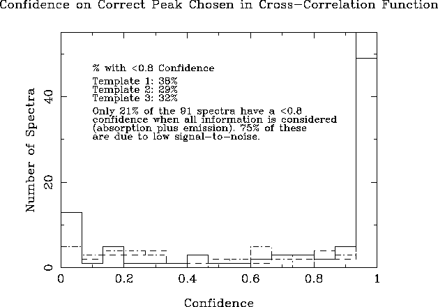
Confidence estimates for the measured redshifts. The sample consists of 91 E/S0 galaxy spectra.
Figure 14.16 shows the histogram of confidences derived from the cross-correlations from this sample (Heavens 1993). These confidences quantify our security that the derived redshifts are real, given the height of the chosen CCF peak relative to the background noise. Over 60 of the spectra have at least one template with a significant confidence. Including information from emission lines, only 21 galaxies, all with signal-to-noise ratio well below that of our faintest galaxies (cf. Figure 3.4.2), had no confident redshift determination.
The duties of the operational database system may be divided into three main subsystems:
The flow diagram for the Operational Data Base
The operational database system is based on the commercial object-oriented data base system "Objectivity". The interface to the OPDB is supported by the C and TCL-based "DERVISH/SHIVA" interactive programming system developed at Fermilab and Princeton. Currently the system will run on a 6-CPU Silicon Graphics Challenge machine with about 60-100 GBy of spinning disk and access to a hierarchical storage tape robot with 3-TB of on-line secondary storage. Tertiary storage of 12-24 TB is in the form of racks of "DLT" high-density tapes. Data is transferred from the mountain top to Fermilab for processing on DLT tapes.
The completed operational database system has basically been delivered as of Fall 1996. The designing data model is complete, the interfaces to all the pipelines have been defined and the code to stage the data into and out of the database in a systematic fashion is implemented.
This process includes all operations that occur between the output of the photometric pipeline and the sending of drilling coordinates to the plate vendor. Operations are performed only on the object catalogs. The following steps are involved:
At this stage, the object lists, flags and other ancillary information are exported to the Science Database.
After a spectroscopic run is made, the reduced spectra, redshifts etc., are also stored in the data bases, together with yet more flags; those linking them to their photometric objects, and those which describe failures of the spectroscopic observations, due to eventualities such as broken fibers, inadequate signal to noise ratio to obtain a useful spectrum, and so on. There is further discussion of the flags and data base objects in Appendices C and D.
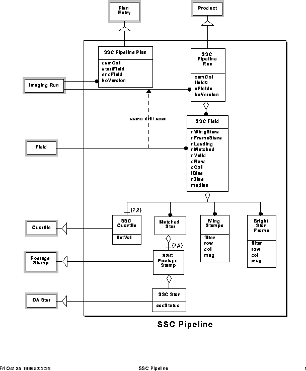
Data model for the SSC pipeline
The software inputs and outputs are tracked with a data model, which is the unique definition of the retained data in the Survey. The data model also defines the interface data between independent components of the Survey (e.g. between separate pipelines, or between pipelines and the operational data base). All pipelines, as well as the operational data base, must be in compliance with the data model. The formal methodology is that of Rumbaugh et al. (1991). The data model is essentially complete for the Monitor Telescope, the DA for the imaging arrays, and the main imaging pipelines. An example, for the SSC, is shown in Figure 14.18. The model is under development for target selection and spectroscopy.
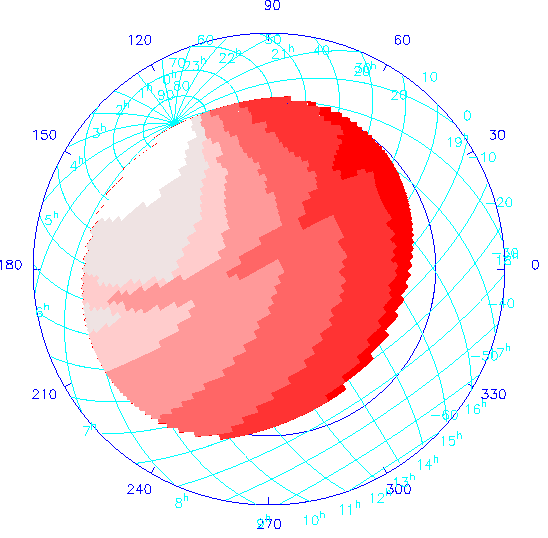
Opportunity weights for the SDSS Northern Survey. Red areas are available less often, white areas more often. The feature through the middle of the map is due to avoidance of the zenith. Both equatorial and galactic coordinates are shown.
Chapters 5 and 15, Survey Strategy and Operations, describe in detail the planning for how the survey will be run. The survey operations will be assisted by a set of sophisticated software tools, loosely called `survey strategy', which: (1) allow the survey to be conducted in an orderly and efficient manner, i.e. ensure that the observing time is efficiently used and that the entire survey time-to-completion is as short as possible. This means that we do not find ourselves, for example, complete except for a few very hard to get pieces of sky, or doing things like always observing at at an airmass of two; (2) monitor the progress of the survey and do the necessary bookkeeping; and (3) allow the total time to completion of the survey to be estimated given assumptions about the weather, etc. At present, we have thoroughly explored the time-to-completion for the Northern imaging survey using these tools (Richards 1996).
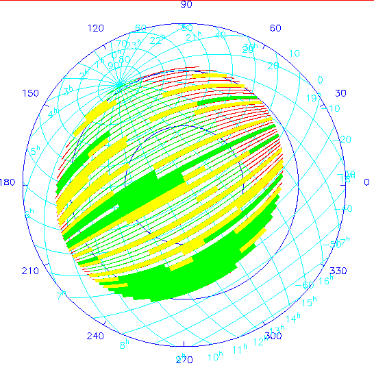
Completed part of the Northern imaging survey after one year. The survey stripes are outlined in red, and those which can be done at sun/moon rise/set "tonight" are overplotted in green. Complete strips are yellow and complete stripes green. Both equatorial and galactic coordinates are plotted.
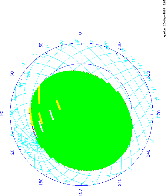
Completed part of the Northern imaging survey after four years. See caption for Figure 14.20.
The software has been used to carry out a series of long-term strategy simulations based on the assignment of opportunity weights to the SDSS Northern area. This map, shown in Figure 14.19, is based on airmass, availability for observation throughout the year, and assumptions about the amount of time lost to bad weather.
The code is then used to investigate how much of the survey will be completed after a given elapsed time under further assumptions about the minimum scan length which is to be observed, night-to-night weather correlations, maximum allowed airmass during a scan (this is a function of the stripe declination, but the goal is to observe as close to the meridian as possible), and so on. The algorithm works roughly as follows. For a given night, the code checks to see which strips have not yet been observed. It then determines how long a scan can be made for each of these strips, given the sidereal time through the night. "Points" are then awarded to each possible scan according to: length (the longer the better); whether the stripe is next to one already done; whether the other strip of the stripe has been done; the stripe's opportunity weight; and whether the entire length of a strip can be done "tonight". It then selects the strip with the best score. If several strips have similar scores, the strip with the lowest opportunity weight is selected to be observed "tonight". The survey time to completion can then be computed by running the code until all observations have been made, on the assumption that all observations are successful. Two examples are shown in Figures 14.20 and 14.21. These figures show the amount of the imaging survey which has been completed in one year and in four years if the APO weather statistics are as described in Chapter 7 and the weather is uncorrelated from night to night. The simulations show that, depending on how the weights are varied and on assumptions about the weather, the times to completion of the imaging survey (not much shorter than the entire time to completion) range from 3.5 to 5.2 years.
The intent of this project is to make the survey data available to the astronomical community in a timely fashion. We currently plan to distribute the data from the first two years of the survey no later than two years after it is taken, and the full survey no later than two years after it is finished. The first partial release may or may not be in its final form, depending on our ability to calibrate it fully at the time of the release. The same remarks apply to the release of the full data set, but we expect the calibration effort to be finished before that release.
Basically, the full set of data in the operational databases will be made available for scientific use by members of the collaboration and for public distribution. The data will likely be reformatted, restructured, and compressed from the operational databases. In addition, the imaging data will be further processed to provide the following products:
The two largest databases, the corrected pixel map and the merged pixel map, are candidates for distribution using wavelet transform compression, whereby the photometric integrity and resolution are preserved at high compressions at the price of not properly recording the noise. Compressions of order 20 are to be had by this technique, which for the merged map (the one of probable interest) reduces to 400 GBy. This, at 700 CD-ROMs, still seems a bit excessive, but there may well be more capacious inexpensive media by the time it exists. The compression technique also has the advantage that there is an accompanying residual file, or a set thereof, successive ones of which add a bit to the reconstruction of the original data and all of which reconstruct it with no loss, but the total is, of course, about the same size as the losslessly compressed database. An alternative to this is to publish a `sky map' with the objects (all of which are fully represented in the atlas) excised or subtracted out, at significantly lower resolution. If we bin 4 x 4 and rescale (for better intensity resolution), we have 1.6 arcsecond resolution, and achieve a reduction of a factor of 16 in data volume. In addition, the data are almost all indistinguishable from sky, and should compress by our normal techniques a factor of very nearly 4, so that the compressed data occupies only 120 GBy or 200 CD-ROMS.
A word is in order about the atlases, their sizes and contents. We have done experiments on faint stars and galaxies in other data and on our Hercules cluster simulations (Figure 3.4.1) for the survey, and have arrived at a subframe size which typically contains all the statistically significant parts of a galaxy; one typically needs a square region
pixels on a side. This is only a guideline, of course, and individual objects will have this dimension individually determined. With the numbers in Table 3.4.1 and the observation that galaxies typically cross the 5:1 signal-to-noise threshold at about g' = 22.5 , we have 5 x 10⁷ galaxies and 7x 10⁷ stars in the survey region, at that S/N cutoff. There are 1.7x 1010 pixels associated with these. There are 2 bytes per pixel and five colors, which comes to 170 GBy. It would be prudent to include a surrounding area at lower resolution to allow following any faint features which might exist, and the overhead is only 19% to include the periphery in a box twice as big but averaged over 4 pixels, i.e. 1.6 arcseconds. This brings the total to 200 GBy, about 2.5% of the whole merged pixel map. Another set of estimates have been made recently from the simulation catalogs (Chapter 13) which also give a number which is 3 to 4% of the sky. In all these cases, the criterion is that the region should include an annulus of width about half its radius which is large enough that the ratio of total object signal in it to sky noise is about unity; any larger one clearly does not, on average, contain significant object data. We have rather arbitrarily chosen a value of 3% areal coverage to arrive at the figures in Table 14.2.
The vast majority of these data are, at the one pixel level, indistinguishable from sky, so the lossless compression factor should be between 3 and 4. Thus the compressed total should be about 80 GBy. The atlas of objects found in the scans is about 1.5 times bigger because of the overlaps, and includes important consistency checks in that a large fraction of the objects will have been observed twice.
There is some question about how to handle objects for the atlas which our classifier thinks are stars; one way which seems satisfactory is to store the parameters of the fitted PSF, subtract it, and make a (highly compressible) image of the residuals at lower resolution. Since there are more stars than galaxies in the sample, doing this in an efficient way is quite important.
The catalogs must be treated very carefully if the amount of data is not to be overwhelmingly large. For all objects, we will want to record positions, at least crude radial profile information in 5 bands from which aperture and isophotal fluxes can be constructed, shape parameters, and pointers to atlas image and calibration information. All told we expect about 250 bytes of information per object, but this may well change as we learn more. One may want to store more for the brighter objects, but their numbers are small and should not increase the total catalog size significantly. The strip scan catalog will be 50% bigger.
It is premature to make firm plans for the form of the public distribution, but we can envisage a multi-level distribution based upon CD-ROMs, which might look something like Table 14.2. In this table, the higher levels correspond to wider anticipated distribution, perhaps with levels <= 0 stored only in the master archive at Fermilab.
| Level | Content | Size | Compressed Size | No. CD-ROMs |
|---|---|---|---|---|
| 3 | Parameter list of Objects with spectra | 750 MBy | 400 MBy | 1 |
| 2 | Parameter list of all objects | 25 GBy | 15 GBy | 25 |
| 1 | Atlas Images | 250 GBy | ~80 GBy | ~130 |
| 1 | Spectra | 50 GBy | 25 GBy | 40 |
| 1 | Sky Map | 500 GBy | 120 GBy | 200 |
| 0 | Flattened 2D Spectroscopic Frames | 70 GBy | 35 GBy | |
| -1 | Merged Pixel Map | 8 TBy | <3 TBy | |
| -2 | Raw data, strips, and scans | 12 TBy | <5 TBy |
It must be kept in mind that it may be possible and most convenient by the time the data are ready to maintain a public-access archive over the successor to the Internet, which circumvents the distribution problem completely and allows easy maintenance of software, though we would probably still want to make some software available for investigators who wish to copy some part of the archive to their own systems. Examples of such software might be routines to uncompress an atlas image into a FITS tape image file or other standard image format, to do the same for some area of the merged pixel map, etc. We are planning to look carefully at the database aspects of the survey catalog data (sorting, keys, etc.), but have not decided at this time what level of support we will offer. At the very least we will supply software to allow reading the catalogs, which will likely be stored in highly compressed binary form.
The production system consists of the individual data processing pipelines integrated together into a cohesive data processing system plus the hardware needed to run that system in routine operation. It also provides the infrastructure needed to allocate resources, schedule and track data processing jobs, store output data sets, and provide mechanisms for dealing with abnormal conditions.
The data flow between all of the major data processing pipelines was shown in Figure 14.3.
The hardware requirements were determined by conducting benchmark tests on the time-intensive sections of pipeline code and by requiring that we be able to turn around a night of imaging or spectroscopic data in 24 hours.
We have purchased three major machines. Two are DEC Alphaserver 8200 5/300 systems. Each has 5 300 MHz processors plus 1 GBy of memory. The third system is an SGI Challenge with 6 150 MHz processors and 512 MBy of memory. We expect to have 300 GBy or more of disk storage distributed among the three systems for the first year of operations, plus several DLT 4000 tape drives. We shall use the two DEC machines for production processing of the imaging and spectroscopic data. The SGI Challenge will hold the object catalog databases and will be used for post-pipeline activities such as quality analysis, merging of object lists, target selection, and distribution of data to collaboration members. In addition, we have access to a hierarchical tape storage system at Fermilab. This system consists of a tape library (maximum capacity of 30 TBy), disk caches, and a file management system. For the first year of operations we plan to utilize 1 - 3 TBy of storage capacity in this system.
All computing systems and the hierarchical tape system will be connected by an FDDI network, which can transfer data at approximately 12 MBy per second.
The major output from the pipelines will consist of corrected frames, the object catalogs, the atlas images, and the 1-D spectra. We expect to hold the object catalogs and 1-D spectra spinning on disk at all times. It is unclear if the atlas images will be kept spinning as well. The corrected frames will be archived to DLT 4000 tapes and will also be transferred to the tape library.
The software needed to operate the production system is not yet developed, since it requires that pipelines be close to their final form. However, the architecture will mimic the standard Fermilab "farms" architecture for processing high energy physics data. The spectroscopic and imaging pipelines, which are the most CPU intensive by far, are designed to process data in discrete, independent "events". For spectroscopy, an "event" consists of all frames pertaining to a single spectroscopic field of 640 fibers. The imaging data from the photometric CCDs is already divided into 6 independent streams, one for each column of CCDs. Each stream is further divided into "fields", each one consisting of 5 frames in the 5 colors of the same area of sky. As an imaging tape is read, each field of 5 frames is assembled and appended with overlapping data from the next field so that each field can be processed as an independent entity. By organizing the data in this fashion, it is possible to have multiple copies of each pipeline running in parallel, with events "farmed" to the next pipeline that becomes idle. At present we expect to stage all outputs from a processing run to disk, so there is no need to require that pipelines deliver their output synchronously (such as would be required if we were writing directly to tape), although such capability could be added if needed.
The following steps will be followed to process imaging data.
Eight tapes are created at APO - 6 Photometric Data tapes from the photometric cameras, 1 2.5M tape with all files produced by the online system (quartiles, star parameters, etc) plus observing log, and 1 MT data tape with all data from the Monitor Telescope.
Tapes are shipped to Fermilab via commercial express carrier
Unpack and label tapes and record in a log
Untar the 2.5M and MT tapes
Create operational database entries for each SDSS imaging run
Create processing plans for the following steps
Process MT data. This step can be done in parallel with the next three
Mount 6 photometric data tapes. Run the SSC pipeline.
Run primary and secondary astrometric calibrations
Review outputs. Create processing plan for photometric data processing
Run postage stamp pipeline
Run photometric frames pipeline on photometric data tapes
Write output corrected images to two sets of tapes and to tape robot.
Write object catalogs to database.
Select a set of imaging runs. For each run, determine acceptable start and stop limits
Run Merge Objects operation
Distribute objects to Science Database
Select targeting area of sky
Set target selection parameters
Run target candidate selection code
Run tiling
Run remainder of target selection code
Define observing conditions
Run plate design code
One tape will be created at APO per night that contains all data.
Tapes are shipped to Fermilab via commercial express carrier
Unpack and label tapes and record in a log
Untar the tape
Create operational database entries for each spectroscopic field observation
Create processing plans for the following steps
Process data through IRAF to perform 2-D extractions and wavelength calibrations
Process 1-D spectra through spectroscopic pipeline
Write parameters to operational database
Write 2-D frames and 1-D spectra to tape robot
Distribute parameters to Science Database
The software effort is large, and is spread among widely geographically separated institutions; it is a challenge to track the progress of the software on a routine basis and to coordinate all of the activities and people involved. Further, as noted above, it is via this software development that much of the astronomical expertise of the collaboration scientists is incorporated into the survey design. Accordingly, we have set up a series of regular meetings and reviews to track and plan the effort.
The development of each major pipeline is coordinated and managed by a responsible individual at the institution. Generally, the pipeline developers hold regular weekly meetings.
This group consists of the pipeline coordinators and the scientific working group chairs, and meets at Fermilab for two days at intervals of 4-6 weeks.
This is held every week at Fermilab with the pipeline coordinators participating by telephone hookup, and focuses on Fermilab software issues, coding standards, framework development etc.
The individual software systems, the integrated software, and the plan for the data acquisition hardware have all received major reviews involving outside participants.
The minutes of all meetings are archived, as are the software requirements documents. In addition, the SDSS has set up a large number of email exploders, maintained and archived at Princeton. These were originally set up to make general announcements and to track progress and milestones in the development of the individual pipelines. Since then further mailing lists were set up for the discussion of scientific issues and progress, and they have expanded yet further to discuss work on several pieces of hardware.
Collins, C.A., Guzzo, L., Nichol, R.C., and Lumsden, S.L. 1995, MNRAS 274, 1071.
Connolly, A.J., Szalay, A.S., Bershady, M.A., Kinney, A.L., and Calzetti, D. 1995, AJ 110, 1071.
de Vaucouleurs, G. 1948, Ann. d'Astroph. 11, 247.
Fukugita, M., Ichikawa, T., Gunn, J.E., Doi, M., and Shimasaku, K. 1996, AJ 111, 1748.
Heavens, A.F. 1993, MNRAS 263, 735.
Kepner, J.V., Fan, X., Bahcall, N.A., Gunn, J.E., and Lupton, R.H. 1997, in preparation.
Lupton, R.H. 1993-1996, "Image Processing in the SDSS: Algorithms", SDSS Internal Documents.
Press, W.H., and Rybicki, G.B. 1993, in `Time Series Prediction: Forecasting the the Future and Understanding the Past', eds. A.S. Weigand and N.A. Gershenfield, SFI Studies in the Science of Complexity, Proc. Vol. XV (Addison-Wesley), 493.
Richards, G. 1996, SDSS Internal Memorandum.
Rumbaugh, J., Blaha, M., Premerlani, W., Eddy, F., and Lorensen, W. 1991, `Object Oriented Modeling and Design', (Prentice-Hall, NJ).
Tonry, J., and Davis, M. 1979, AJ 84, 1511.